This post discusses the problem of the gambler’s ruin. We start with a simple illustration.
Two gamblers, A and B, are betting on the tosses of a fair coin. At the beginning of the game, player A has 1 coin and player B has 3 coins. So there are 4 coins between them. In each play of the game, a fair coin is tossed. If the result of the coin toss is head, player A collects 1 coin from player B. If the result of the coin toss is tail, player A pays player B 1 coin. The game continues until one of the players has all the coins (or one of the players loses all his/her coins). What is the probability that player A ends up with all the coins?
Intuitively, one might guess that player B is more likely to win all the coins since B begins the game with more coin. For example, player A in the example has only 1 coin to start. Thus there is a 50% chance that he/she will lose everything on the first toss. On the other hand, player B has a cushion since he/she can afford to lose some tosses at the beginning.
___________________________________________________________________________
Simulated Plays of the Game
One way to get a sense of the winning probability of a player is to play the game repeatedly. Rather than playing with real money, why not simulate a series of coin tosses using random numbers generated in a computer? For example, the function =RAND() in Excel generates random numbers between 0 and 1. If the number is less than 0.5, we take it as a tail (T). Otherwise it is a head (H). As we simulate the coin tosses, we add or subtract to each player’s account accordingly. If the coin toss is a T, we subtract 1 from A and add 1 to B. If the coin toss is an H, we add 1 to A and subtract 1 from B. Here’s a simulation of the game.
Image may be NSFW.
Clik here to view.
In the first simulation, player A got lucky with 4 heads in 5 tosses. The following shows the next simulation.
Image may be NSFW.
Clik here to view.
Player A seems to be on a roll. Here’s the results of the next two simulated games.
Image may be NSFW.
Clik here to view.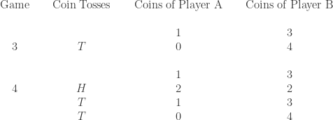
Now player A loses both of these games. For good measure, we show one more simulation.
Image may be NSFW.
Clik here to view.
This one is a little more drawn out. Several tosses of tail in a row spells bad news for player A. When a coin is tossed long enough, there bounds to be some runs of tails. Since it is a fair coin, there bounds to be runs of head too, which benefit player A. Wouldn’t the runs of H cancel out the runs of T so that each player wins about half the time? To get an idea, we continue with 95 more simulations (to get a total of 100). Player A wins 23 of the simulated games and player B wins 77 of the games. So player A wins about 25% of the times. Note that A owns about 25% of the coins at the start of the game.
The 23 versus 77 in the 100 simulated games may be just due to luck for player B. We simulate 9 more runs of 100 games each (for a total of 10 runs with 100 games each). The following shows the results.
-
Ten Simulated Runs of 100 Games Each
Image may be NSFW.
Clik here to view.

The simulated runs fluctuate quite a bit. Player A wins any where from 19% to 34% of the times. The results are no where near even odds of winning for player A. In the 1,000 simulated games, player A wins 24.6% of the times, roughly identical to the player A’s share of the coins at the beginning. If the simulation is carried many more times (say 10,000 times or 100,000 times), the overall winning probability for player A would be very close to 25%.
___________________________________________________________________________
Gambler’s Ruin Problem
Here’s a slightly more general description of the problem of gambler’s ruin.
Gambler’s Ruin Problem
Two gamblers, A and B, are betting on the tosses of a fair coin. At the beginning of the game, player A has Image may be NSFW.
Clik here to view.
Clik here to view.
Clik here to view.
Solution: Gambler’s Ruin Problem
The long run probability of player A winning all the coins is Image may be NSFW.
Clik here to view.
The long run probability of player B winning all the coins is Image may be NSFW.
Clik here to view.
In other words, the probability of winning for a player is the ratio of the number of coins the player starts with to the total numbers of coins. Turning it around, the probability of a player losing all his/her coins is the ratio of the number of coins of the other player to the total number of coins. Thus the player with the fewer number of coins at the beginning has a greater chance of losing everything. Think a casino. Say, it has 10,000,000 coins. You, as a gambler, have 100 coins. Then you would have a 99.999% chance of losing all your coins.
The 99.999% chance of losing everything is based on the assumption that all bets are at even odds. This is certainly not the case in a casino. The casino enjoys a house edge. So the losing probabilities would be worse for a gambler playing in a casino.
___________________________________________________________________________
Deriving the Probabilities
We derive the winning probability for a more general case. The coin that is tossed does not have to be a fair coin. Let Image may be NSFW.
Clik here to view.
Clik here to view.
Clik here to view.
Let Image may be NSFW.
Clik here to view.
Clik here to view.
Clik here to view.
Clik here to view.
Clik here to view.
Clik here to view.
Clik here to view.
Clik here to view.
The goal here is to derive expressions for both Image may be NSFW.
Clik here to view.
Clik here to view.
Clik here to view.
Clik here to view.
Another point to keep in mind is that we can assume Image may be NSFW.
Clik here to view.
Clik here to view.
Clik here to view.
Clik here to view.
Clik here to view.
Clik here to view.
Let Image may be NSFW.
Clik here to view.
Clik here to view.
Clik here to view.
Clik here to view.
-
Image may be NSFW.
Clik here to view.

Consider the conditional probabilities Image may be NSFW.
Clik here to view.
Clik here to view.
Clik here to view.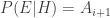
Clik here to view.
Clik here to view.
Clik here to view.
Clik here to view.
-
Image may be NSFW.
Clik here to view.

Further derivation can be made on equation (2).
Image may be NSFW.
Clik here to view.

Image may be NSFW.
Clik here to view.

Image may be NSFW.
Clik here to view.

Plugging in the values Image may be NSFW.
Clik here to view.
Clik here to view.
Clik here to view.
Image may be NSFW.
Clik here to view.
![\displaystyle \begin{aligned} &A_{2}-A_{1}=\frac{q}{p} \ (A_1-A_{0})=\frac{q}{p} \ A_1 \\&A_{3}-A_{2}=\frac{q}{p} \ (A_2-A_{1})=\bigg[ \frac{q}{p} \biggr]^2 \ A_1 \\&\ \ \ \cdots \\&A_{i}-A_{i-1}=\frac{q}{p} \ (A_{i-1}-A_{i-2})=\bigg[ \frac{q}{p} \biggr]^{i-1} \ A_1 \\&\ \ \ \cdots \\&A_{n}-A_{n-1}=\frac{q}{p} \ (A_{n-1}-A_{n-2})=\bigg[ \frac{q}{p} \biggr]^{n-1} \ A_1 \end{aligned}](http://s0.wp.com/latex.php?latex=%5Cdisplaystyle+%5Cbegin%7Baligned%7D+%26A_%7B2%7D-A_%7B1%7D%3D%5Cfrac%7Bq%7D%7Bp%7D+%5C+%28A_1-A_%7B0%7D%29%3D%5Cfrac%7Bq%7D%7Bp%7D+%5C+A_1+%5C%5C%26A_%7B3%7D-A_%7B2%7D%3D%5Cfrac%7Bq%7D%7Bp%7D+%5C+%28A_2-A_%7B1%7D%29%3D%5Cbigg%5B+%5Cfrac%7Bq%7D%7Bp%7D+%5Cbiggr%5D%5E2+%5C+A_1+%5C%5C%26%5C+%5C+%5C+%5Ccdots+%5C%5C%26A_%7Bi%7D-A_%7Bi-1%7D%3D%5Cfrac%7Bq%7D%7Bp%7D+%5C+%28A_%7Bi-1%7D-A_%7Bi-2%7D%29%3D%5Cbigg%5B+%5Cfrac%7Bq%7D%7Bp%7D+%5Cbiggr%5D%5E%7Bi-1%7D+%5C+A_1+%5C%5C%26%5C+%5C+%5C+%5Ccdots+%5C%5C%26A_%7Bn%7D-A_%7Bn-1%7D%3D%5Cfrac%7Bq%7D%7Bp%7D+%5C+%28A_%7Bn-1%7D-A_%7Bn-2%7D%29%3D%5Cbigg%5B+%5Cfrac%7Bq%7D%7Bp%7D+%5Cbiggr%5D%5E%7Bn-1%7D+%5C+A_1+%5Cend%7Baligned%7D&bg=ffffff&fg=333333&s=0&c=20201002)
Adding the first Image may be NSFW.
Clik here to view.
-
Image may be NSFW.
Clik here to view.
![\displaystyle A_i-A_1=A_1 \ \biggl[\frac{q}{p}+\bigg( \frac{q}{p} \biggr)^{2}+\cdots+\bigg( \frac{q}{p} \biggr)^{i-1} \biggr]](http://s0.wp.com/latex.php?latex=%5Cdisplaystyle+A_i-A_1%3DA_1+%5C+%5Cbiggl%5B%5Cfrac%7Bq%7D%7Bp%7D%2B%5Cbigg%28+%5Cfrac%7Bq%7D%7Bp%7D+%5Cbiggr%29%5E%7B2%7D%2B%5Ccdots%2B%5Cbigg%28+%5Cfrac%7Bq%7D%7Bp%7D+%5Cbiggr%29%5E%7Bi-1%7D+%5Cbiggr%5D&bg=ffffff&fg=333333&s=0&c=20201002)
Image may be NSFW.
Clik here to view.
![\displaystyle A_i=A_1 \ \biggl[1+\frac{q}{p}+\bigg( \frac{q}{p} \biggr)^{2}+\cdots+\bigg( \frac{q}{p} \biggr)^{i-1} \biggr] \ \ \ \ \ \ \ \ \ \ \ \ \ \ \ \ \ \ \ \ \ \ \ \ \ \ \ (3)](http://s0.wp.com/latex.php?latex=%5Cdisplaystyle+A_i%3DA_1+%5C+%5Cbiggl%5B1%2B%5Cfrac%7Bq%7D%7Bp%7D%2B%5Cbigg%28+%5Cfrac%7Bq%7D%7Bp%7D+%5Cbiggr%29%5E%7B2%7D%2B%5Ccdots%2B%5Cbigg%28+%5Cfrac%7Bq%7D%7Bp%7D+%5Cbiggr%29%5E%7Bi-1%7D+%5Cbiggr%5D+%5C+%5C+%5C+%5C+%5C+%5C+%5C+%5C+%5C+%5C+%5C+%5C+%5C+%5C+%5C+%5C+%5C+%5C+%5C+%5C+%5C+%5C+%5C+%5C+%5C+%5C+%5C+%283%29&bg=ffffff&fg=333333&s=0&c=20201002)
There are two cases to consider. Either Image may be NSFW.
Clik here to view.
Clik here to view.
Clik here to view.
Clik here to view.
Clik here to view.
Image may be NSFW.
Clik here to view.
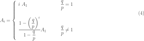
The above two-case expression for Image may be NSFW.
Clik here to view.
Clik here to view.
Clik here to view.
Clik here to view.
Clik here to view.
Clik here to view.
Image may be NSFW.
Clik here to view.

Plugging Image may be NSFW.
Clik here to view.
Image may be NSFW.
Clik here to view.

The expression for Image may be NSFW.
Clik here to view.
Clik here to view.
Clik here to view.
Clik here to view.
Clik here to view.
Clik here to view.
Clik here to view.
Image may be NSFW.
Clik here to view.

For the case Image may be NSFW.
Clik here to view.
Clik here to view.
Clik here to view.
Clik here to view.
Clik here to view.
-
Image may be NSFW.
Clik here to view.

The fact that Image may be NSFW.
Clik here to view.
___________________________________________________________________________
Further Discussion
The formulas derived here are quite profound, not to mention impactful and informative for anyone who gambles. More calculations and discussion can be found here in a companion blog on statistics.
___________________________________________________________________________
Image may be NSFW.
Clik here to view.